
 |
 |
|---|
Motivation
The Kalman filter finds applications in extracting useful data from inherently noisy sources. One common application is smoothing sensor data. In order for most sensor data to be effectively employed in applications like control loops or navigation systems it must first be filtered in a manner that removes noise but, does not introduce an unacceptable amount of additional error or increases processing and memory load on the system. In this regard the Kalman filter excels. The Kalman filter can also be extended to combine data from multiple input sources to further reduce the error in a signal or sample. This property has many applications in the area of sensor fusion. Kalman filter sensor fusion is commonly used in robotic control systems. A common use case is autonomous vehicle navigation and control eg. Quadcopters or spacecraft. Additionally, the Kalman filter is often used in analog and digital signal processing. The Kalman filter algorithm enjoys implementations in both software and hardware.
Describe Algorithm details
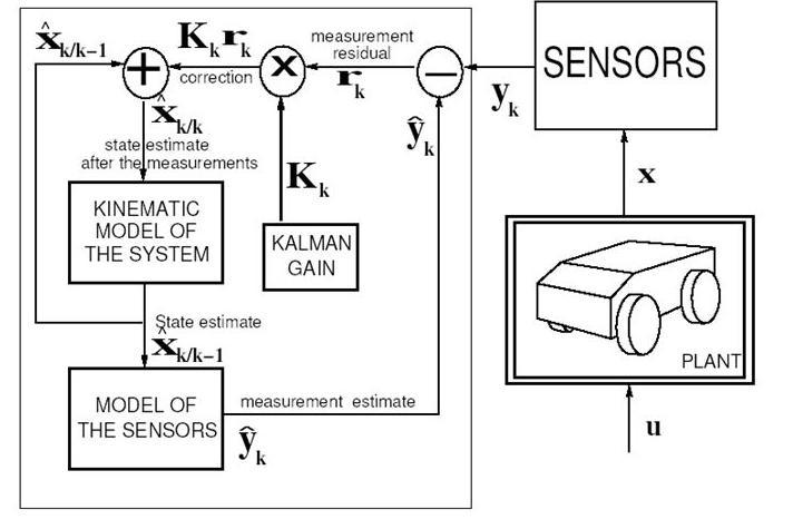
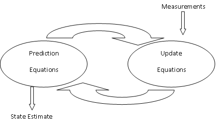
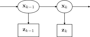
The Kalman filter algorithm uses multiple input signals samples, often periodically, to increase the overall estimation accuracy of the signal with noise removed. The Kalman filter has 5 sets of variables one must understand. The the first is the self-explanatory unfiltered input signal. It is important to state, the algorithm assumes that all input signals into the filter contain a certain amount of noise variance. The Kalman gain, which is recursively calculated from the variance of the input signal over many samples. The last state (Xk-1) of the system, which is a gain weighted sum of all previous input signal samples. The current state (Xk) , which is an estimate of the expected state of the system as calculated by a function that describes the system/signal. The output signal is a gain weighted sum of the value of the current input signal and the current state estimation of the system. The Kalman filter algorithm uses two main components, a predicative step and a update step. See Figure 1.
 |
 |
|---|---|
| Figure 1. Simplified process flow representation of input signal and estimation in kalman filter. |
In the predictive step the Kalman filter relies upon a function model of the system/signal in order to calculate the predicted current state (Xk) from the last state (Xk-1) and any relevant input signals. The system/signal predicted variance is also calculated in this step.
In the update step, the next estimated output signal is produced from a gain weighted sum of the estimated current state and the new input signal sample. In the case of a temperature sensor, the Kalman filter would produce a new estimated temperature for the output from the gain weighted sum of previous temperature samples and the new temperature sample. The gain is calculated based upon the variance observed between the predicted variance and the variance of the new sample. The filter is tuned to give a higher weight to samples with lower error.
Explain why the chosen algorithms are employed for the problem.
The algorithm has found employment as a solution to many common engineering problems such as processing inputs into control systems and for fusing sensor data from multiple sources. The algorithm is popular as a solution to these problems due to its low memory and processing footprint, constant running time, and comparatively simple design as compared to other solutions. The Kalman filter reduces the amount of working memory required by encoding past history of the inputs into a single current state variable (Xk). This encoding reduces the amount of memory consumed by the algorithm as past information does not need to be retained. Additionally, the amount of data processing per signal sample is reduced as only the current state variable and new sample are processed. These reductions in processing and memory are advantages in resource constrained environments, such as embedded systems or hardware implementations. The Kalman filter algorithm also lends itself well to “real time” systems such as robotic control where a predictable delay and constant runtime is required.The Kalman filter algorithm has a O(1) processing complexity and a O(1) memory space complexity. The Kalman filter can also be extended to combine inputs from multiple sources to further reduce signal sample variance. This property lends itself well to applications employing sensor fusion such as inertial navigation units (INUs)
Experimental configuration and details.
The experiment consists of a force sensitive resistor sensor sampled once every 100 mSec by an Arduino compatible microcontroller(ESP8266). The microcontroller sends the raw sensor samples to the computer over a serial connection. The computer then writes the raw samples to a file on the hard disk (Data.txt). Once a large number of samples have been collected, the raw samples are passed into the Kalman filter(KalmanFilterWrapper.exe). KalmanFilterWrapper.exe produces two output files KALMAN_INPUT_VS_OUTPUT.csv and KALMAN_FILTER_RUNNING_TIME_VS_INPUT_SIZE.csv that contain the raw samples vs the Kalman filtered samples and the running time vs input size respectively. Kalman filters will often have many sensor inputs , process time variant signals, and must account for control inputs. With the addition of more inputs a gain matrix must be maintained that relates each input to each other input in addition to the gain between current Xk and last state Xk-1. These factors quickly drive a simple algorithm into such a complex system that it is used routinely in PHD. thesi. For these reasons, a simple implementation of the Kalman was chosen. Finally, a simpler implementation will clearly show the algorithm operation. The implemented Kalman filter is processing a single variable, static , time invariant signal(Voltage proportional to the weight of Expo marker) In this implementation, the function model of the system/signal is Current state = last state I.e Xk = Xk-n. The test should clearly show noise in raw samples and the resulting filtered output of the Kalman filter.
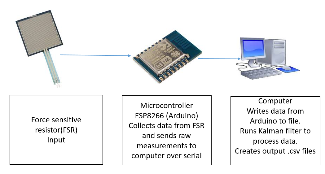
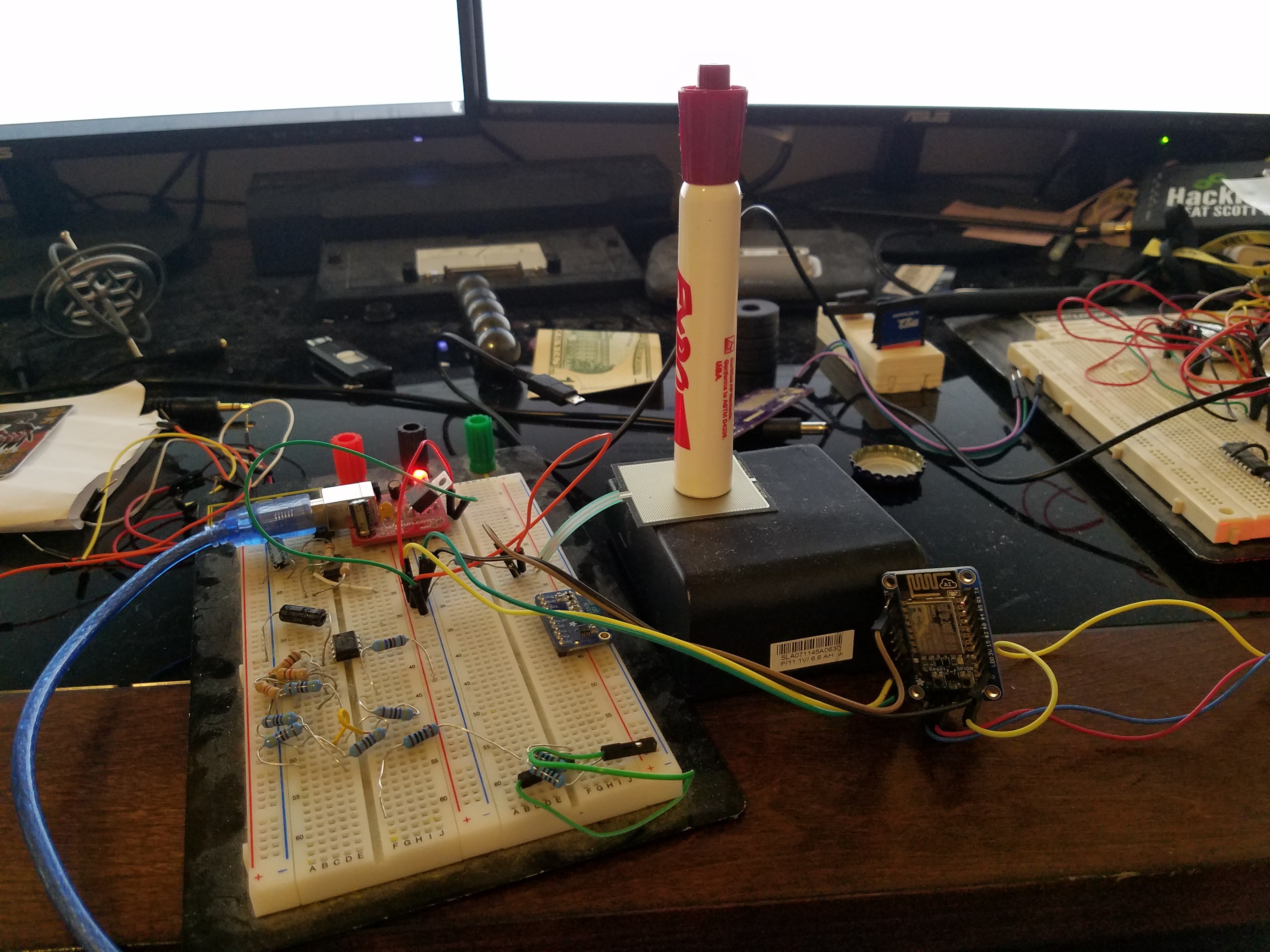
Figure 2: Experimental setup to collect sensor data. EXPO marker used to provide static weight greater than baseline.

Figure 3. Schematic of the circuit used to collect data and send information the the computer.
Source code and related information to reproduce experiment
Arduino code to collect samples:
DataStructuresKalmanFilter.ino
Schematic of sensor collection:
Kalman_sensor_collection_schematic.pdf
Kalman filter Source Code see:
KalmanFilterWrapper.cpp – Wrapper to process data and produce output files
./KalmanFilter.cpp – Kalman filter implementation
Run make in project root to compile C++ source code.
make
Exec KalmanFilterWrapper.exe to produce outfiles
KALMAN_INPUT_VS_OUTPUT.csv
KALMAN_FILTER_RUNNING_TIME_VS_INPUT_SIZE.csv
All code can be found at https://github.com/JohnGrun/KalmanFilterPaper
Sources of Variance in the experiment
Raw measurement sources of known variance
The sensor employed(FSR406) has tolerance of 2% at constant temperature as called out in the data sheet Datasheets_FSR.pdf. At a supply voltage of 3.3v, 2% is ~0.066 Volts of error due to the FSR sensor.See references for link to data sheet.
The Esp8266 ADC has a resolution of 12 bits or 4096 divisions. With a Vcc = 3.3V; 4096 = 3.3 Volts, 0 = 0 Volts. A change of 1 in a measurement corresponds to 3.3/4096 = 0.00080566406 Volts. Compared the 0.066 Volts of error introduced by the FSR sensor the ADC resolution is not seen to be significant and, can thus be neglected in calculations.
Running time sources of known variance
The running time of the algorithm may be influenced by external factors such as file system assess, resource allocations, paging, or process scheduling. To compensate for the aforementioned sources of external variances many samples have to be taken.
Results and Analysis
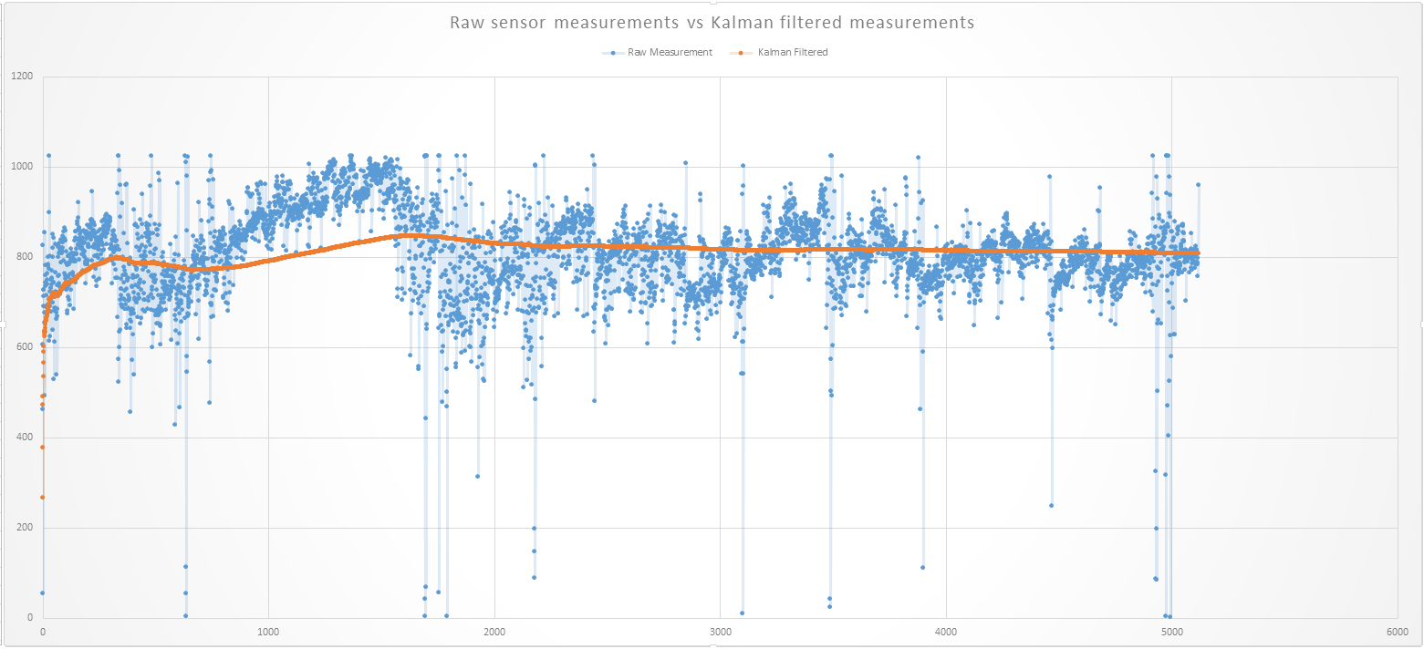
Figure 4. Sensor samples of proportional voltage to weight of EXPO marker. Raw samples from FSR sensor (Blue). Kalman filtered data of samples (Orange).
As can be seen in Figure 4, the raw samples contain a large amount of noise. The standard deviation of the raw samples was 1478.01. A static, time invariant signal( Voltage proportional to the weight of Expo marker) with such a high standard deviation is unusable in real world applications. Once the signal is processed by the Kalman filter, and significant time has passed, the signal become far less variable. The standard deviation of Kalman filtered signal was 98.07, a full order of magnitude less than the raw input signal. Additionally, the filtered signal reached a stable output with low variance as would be expected with a static input signal (Voltage proportional to the weight of Expo marker).
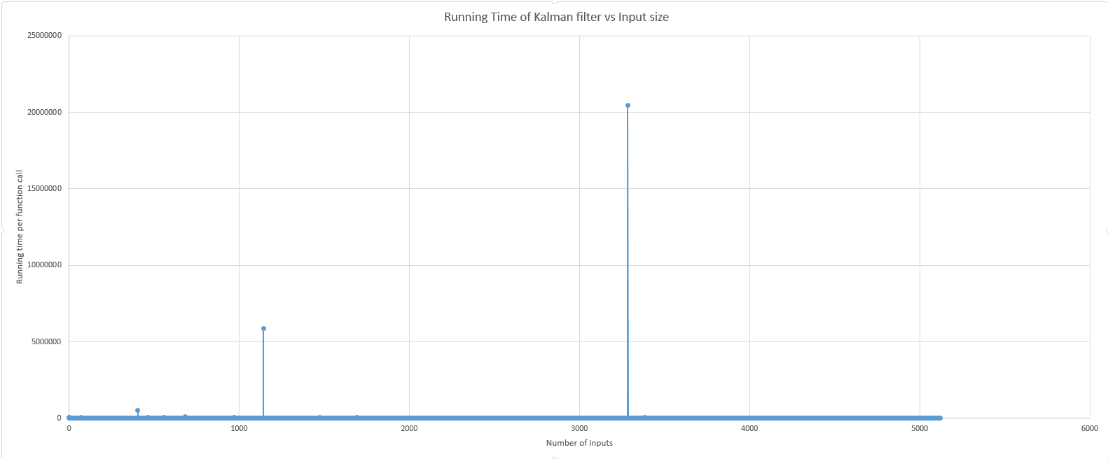
Figure 5. Running Time vs Input size. Running time (Blue) of each call to the Kalman filter algorithm using same data in Figure 4.
The second graph Figure 5. depicts the running time of the Kalman filter vs the number of samples processed. As expected, the running time is O(1). The Kalman filter only processes one measurement at a time. The output estimation is a weighted sum the past state( all previous samples) and the current measurement state and is updated once per function call. Only for 2 data points out of 5121 samples did the running time change significantly. These 2 data points are likely due to other factors not related to the Kalman filter, such as process scheduling or file system assesses on the host computer.
Discussion
As can be seen from the results of the experiments the Kalman filter algorithm manages to clean up a noisy signal while running in constant time. There are two limitations of the Kalman filter algorithm. The algorithm requires a finite amount of startup time to reach a output that is representative of the filtered signal see Figure 4. In practice, as long as this startup time can be tolerated, a valid output signal can be extracted. The other limitation is that the Kalman filter algorithm requires knowledge of the process. This is manifested in the prediction stage, where the value of Xk is based upon an equation describing how the system/signal will change over time. E.g. Xk = F(Xkn-1,input1, input2). This makes it difficult to use a Kalman filter algorithm as general case filter, or where the input signal does not have a known function describing its behavior. If one can tolerate these minor shortcomings the Kalman filter algorithm is an excellent choice to clean up noisy input signals with minimal memory and processing overhead.
References
The Extended Kalman Filter: An Interactive Tutorial for Non-Experts. (2017, April 28). Retrieved April 28, 2017, from https://home.wlu.edu/~levys/kalman_tutorial/kalman_01.html
Kelly, A. (2006, May 24). A 3D State Space Formulation of a Navigation Kalman Filter for Autonomous Vehicles. Retrieved April 3, 2017, from http://www.frc.ri.cmu.edu/~alonzo/pubs/reports/kalman_V2.pdf
Welch, G., & Bishop, G. (2001). An Introduction to the Kalman Filter. Retrieved April 3, 2017, from http://www.cs.unc.edu/~tracker/media/pdf/SIGGRAPH2001_CoursePack_08.pdf
Wikipedia. (2017, April 28). Variance. Retrieved April 3, 2017, from https://en.wikipedia.org/wiki/Variance
Interlink Electronics. (2017, April 4). FS R ® 400 Series Data Sheet. Retrieved April 4, 2017, from https://www.interlinkelectronics.com/datasheets/Datasheet_FSR.pdf
Kohanbash, Y. (2014, January 30). Kalman Filtering – A Practical Implementation Guide (with code!). Retrieved April 29, 2017, from http://robotsforroboticists.com/kalman-filtering/
Wikipedia. (2017, April 06). Kalman filter. Retrieved April 29, 2017, from https://en.wikipedia.org/wiki/Kalman_filter