Broken encoder

I dropped my trusty Rigol scope off of the table while testing. The trigger encoder knob broke off.

Replacement part

After a bit of googling I was able to locate the part number. This is a very popular scope with hobbyist so this information was not all that hard to find.

Opening the case

The screws that hold the case on are Trox or star drive. There are 6 screws. Two screws on the bottom near the feet, two screws under the handle, and two screws on either side of the power socket.

WARNING: Do not forget to remove the power button. If you try the case with the power button still in place the switch will snap off. The power button can be removed by pulling it upwards.

You will need an extension bit to get at the screws under the handle

Do not forget about the screws on the side

Back case removed

Once the case is removed, unscrew the standoffs on either side of the serial interface (DB9).
Lift off the metal rf sheild

You will need to remove all the screws inside of the case. All The power supply board must be removed
Disconnect the power supply board. Watch out for the LCD lamp power cable (Red/White cable with JST connector)

You will need to disconnect the white ribbion cable from the board at the bottom of the unit.

The front case panel can now be removed.

Power supply board. Power switch

Front case panel removed. Picture of the 3 screws holding on the user control board.
These will need to be removed.

Replacing the encoder

Boken encoder next to replacement encoder.

Bottom of the user control board. Unsoldering required.
WARNING: Rigol uses lead free solder. Only use lead free solder. If you mix leaded solder and lead free solder a new alloy with a higher melting point will be formed. Good luck removing that!

Desoldered encoder

Replacement encoder

Put everything back together

Parts

Magnetic Door Latch

3d Printed Magnetic Latch mount

Mounting the Door

Hinges

3d Printed Hinges

Door temporarily held on by clamps. Hinges mounted to the frame. Using a center locating punch through the hing mounting holes to locate where to drill the hole.

Determining the correct drilling points with a punch

Drilling Hinge Mounting Holes.
In this case I tapped the acrylic plate with a 1/4-20 tap. These holes need to be kept away from the edge otherwise breakage can occur. Additionally, spreading the load across many holes reduces the stress on any one hole.

Mounting the door with the hinges
Door mounted with the 1/4-20 bolts

Door Mounted to Hinges

Door Handle

Insert Grub console picture here

run the following commands

• ls

Will show you all the drive parations

(hd0,gpt1)

• ls (hdo,gpt1)/

Will give you a listing of all the files on the dive

• Find the drive that contains /boot

(hd0,gpt1)/boot

• locate the grub.cfg

configfile /PathToFile/grub.cfg

configfile (hd0,gpt1)/boot/grub/grub.cfg

• Grub boot menu should start.

• Kernel is now running

• Fix any broken packages
  dpkg –configure -a

• Check systemctl

• Look for any errors that may have occured.

• Fix any filesystem errors that may have occures

• look in /dev/disk/by-uuid

• Perform fsck on any drives that require a repair.
  fsck /dev/disk/by-uuid/abc456

• Often the grub loader cannot find the efi file

• sudo apt install grub-efi-amd64

Wet/Dry Cough Analysis and Differentiation

Introduction

One symptom that often accompanies an illness is a cough. It has been noted that certain types of coughs are often associated with certain medical conditions. This relationship has led to the practice using coughs to aid in the diagnosage of patients. For this study, we will attempt to differentiate between two common cough categories, Wet and Dry coughs.

A Wet cough is caused by the presence of mucus in the airway. The common causes of a wet cough include cold,flu, pneumonia,chronic obstructive pulmonary disease (COPD), emphysema,chronic bronchitis,acute bronchitis or asthma

A Dry cough is a cough where mucus is not present in the airway. Dry coughs may occur in long fits and are often caused by irritation in the respiratory tract. The common causes of dry coughs include flu, cold, laryngitis, sore throat, croup, tonsillitis, sinusitis, asthma, allergies, or exposure to irritants such as air pollution, dust, mold, or smoke

Background Research

Before analysis began a limited background search was performed. Survey papers in the area of auscultation were consulted to give a general understanding of the current standing of the field and to discover methods to analyze the data. The survey papers listed several methods common within the field including FFT, Spectral Contrast, and MFCC.3 Several papers mentioned additional techniques often applied to music identification such as Chromagraph and Tonnez as possibly relevant to auscultation research. These techniques will be presented in more detail in the Feature Extraction Section. Additional research on the differences between a dry and wet cough and previous wet/dry cough studies were also consulted.

Data Collection

Cough Collection 1

The initial data collection known henceforth as Cough Collection 1 consisted of 24 samples collected in a clinical setting by several doctors volunteering their time. The collection is a mix of wet and dry coughs from both female and male patients. The coughs were recorded in either WAV sampled at 16000 Hz or MP4a sampled at 48000Hz by cell phone applications. Each recording contains multiple coughs. The filename of each cough included a substring denoting gender and cough type. E.g FWC = Female wet cough, MDC = Male dry cough.

Cough Collection 2

After a preliminary analysis was performed on Cough Collection 1 several doctors from UMDNJ deemed the preliminary analysis sufficient to begin a second data collection. The second data collection will be referred to as Cough Collection 2 going forward. The preliminary analysis is presented in a later section of this document. Cough Collection 2 is ongoing and is expected to produce 100 samples. Coughs were collected by a doctor in a clinical setting from both Male and Female patients. Each recording contains multiple coughs. The collection consists of cough recording saved in OPUS format with a sampling rate of 16000 Hz. The file names were changed to reflect the gender and cough type while also matching the file naming convention developed during Cough Collection 1 except files from Cough Collection 2 begin numbering from 200. E.g FWC200, FWC201, MDC200,MWC200. The OPUS files were converted to wav files with a sampling rate of 16000Hz. An excel log was kept to track cough samples as they came in.

Visualizing the Data

Before any analysis was conducted, the data was visualized to gain an understanding of the structure of the data and to perform quality checks.

Data Standardization (Pre processing )

Cough Collections 1 & 2 contained files with differing naming conventions several different audio formats. These inconsistencies were rectified during the standardization process. The file names were renamed into a standardized format of ( Gender Type of Cough Number .extension).

Where:

• Gender = M/F
• Type of Cough = WC/DC
• Number = linearly increasing number.

Example:

• Original Filename = S1.3MDC2.wav
• ` New File name = MDC1.wav

All the files were converted into 16KHZ Mono Wave and the average amplitude of each cough sample was set to -20 db. This amplitude normalization step was required to correctly segment the coughs into individual coughs.

A log was produced that includes the original file name, new file name, and if file conversion was required for a given cough sample.

Segmenting the audio files into separate coughs

Each audio file from Cough collections 1&2 contains multiple coughs. Due to the large number of samples expected, 124 files between Cough Collections 1&2, manual separation was deemed to be untenable. An audio segmenter was written to split each audio file into individual coughs. All audio files were previously set to the same average amplitude level (-20dB) during the standardization step. The files were split where the audio exceeds a threshold. The threshold was determined experimentally.

Full audio file

Audio segment

This method works reasonably well but problems do arise such as segments containing silence, blips, or human voices are sometimes generated. To correct this issue of generating silence and quick blip segments the entire dataset( Cough Collections 1&2) was examined for commonalities between the silence and blip segments. Fortunately , all silence and blip clips were below a certain length and could easily be filtered out automatically. Segments containing human voices can not be automatically identified at this time and must be manually removed. For this reason, manual inspection of the audio segments is still recommended at this time.

Data Augmentation

Data augmentation is the process of artificially expanding a data set by means of transforms. These transforms may take the form of shifting, cropping, scaling or etc. Data augmentation can also change the data set to be more representative of the problem of interest by introducing variations that are not represented in the unaugmented dataset. In this study the cough files are standardized to the same length (frame) to match the input size of the algorithms used but a cough may occur at any point within the frame. By using time shifting augmentation several samples of cough can appear in different regions of the frame. This time shifting within a frame can have the effect of desensitizing an algorithm to a temporal dependency that does not have bearing on if a cough is wet or dry.

Issues with data augmentation

Data augmentation does come with some shortfalls. Each new generated sample is similar to another sample present within the existing data set. As a higher percentage of the data set becomes augmented, the data set will start to exhibit similarities that may not be as pronounced outside of the augmented dataset. This effect is more apparent on very small datasets which may not be an accurate representative subset of the larger problem of interest. E.g Cough samples from a very small set of individuals may exaggerate frequency components that may not be as dominant in the general population. E.g A dataset containing only male coughs. In the context of a machine learning classifier, the prediction accuracy may increase on similar samples but will fail to generalize well on samples that are not as similar to the original samples.

The correct level of data augmentation and application is a current active research topic. For this study, only established methods were employed and augmented data was limited to representing 80% of the entire dataset. As more samples were introduced, the level of augmentation was reduced. Two types of data augmentation were used in this study, time shifting and adding white noise.

Female Dry Cough Raw Audio

Time Shifted Female Dry Cough

Female Dry Cough with additional White Noise

Feature extraction

Feature extraction is the process of applying transforms to data to gain insight into the structure of the data, or to find similarities or differences between samples of the data. It can also serve as a method of dimensional reduction or to convert data from one format to another. E.g Audio to image files. The features investigated in this study are shown below.

Mel-frequency cepstrum (MFCC)

The mel-frequency cepstrum (MFCC) is a representation of the short-term power spectrum of a sound, based on a linear cosine transform of a log power spectrum on a nonlinear mel scale of frequency.
Female Dry cough

Female Wet Cough

Male Dry Cough

Male Wet Cough

Spectrogram
A spectrogram is a visual representation of the spectrum of frequencies of a signal as it varies with time. Spectrograms are able to capture both frequency and temporal information about a signal.

Female Dry Cough

Female Wet Cough

Male Dry Cough

Male Wet Cough

FFT Squared or FFT Magnitude

FFT Magnitude is a common technique used to drive down the noise floor in the FFT while accenting the main frequency components of the signal.

Female Dry Cough

FFT Magnitude of same Female Dry Cough

Chromagram

The entire spectrum of the audio signal is projected onto 12 bins representing the 12 distinct semitones (or chroma) of the musical octave. The chromagram was included in the librosa library employed in this study and was implemented for no extra effort.

Chromagram of Female Dry Cough

Spectral Contrast
Represents the relative spectral distribution instead of average spectral envelope power.

Spectral Contrast of Female Dry Cough

Tonnetz

Tonnetz or tone-network is a lattice diagram that represents the tones of western music within a space. Tonnetz is useful for analysing the tonal content of an audio sample. While often used for analysing the structure of music, torrentz was investigated in addition to the other features as it detects the changes in the harmonic content of audio signals that may be useful in differentiating wet from dry coughs. Torrentz was included in the librosa library employed in this study and was implemented for no extra effort.

Tonnetz of Female Dry Cough

Data Processing Pipeline

The following diagram shows a high level overview of the flow of data within the software

• Load files into memory as dictionary of numpy arrays
• The dictionary format
  • Key = Set Name
  • Value = nxm numpy matrix
  • N = # of files in set
  • M = Samples in each audio file
• The dictionary can be fed into Data Augmentation then into Feature Extraction or directly into the Feature Extraction. The feature extraction block creates a new dictionary containing numpy arrays of the extracted features. The new dictionary is of the same format as the input dictionary.
• Once features of interest have been extracted the data can analyzed.

Preliminary Analysis

Before the time investment could be justified to collect additional samples (Cough Collection 2) a preliminary analysis had to be conducted. The goal of this preliminary analysis was to attempt to differentiate a Wet Cough from a Dry Cough with the samples from Cough Collection 1.

Wet and dry coughs were separated into two sets, one set contains all wet coughs while the second set contains all dry coughs.

The Preliminary Analysis was based upon the following Hypothesis;

To differentiate Wet and Dry Coughs we must be able to prove each set is more similar to itself than to the other sets. I.E. A wet cough is more similar on average to another wet cough than to a dry cough. This implies that the average correlation within a set must be greater than the average correlation between different sets.

Procedure

Before the preliminary analysis could begin, some preprocessing steps had to be accomplished. First, each of the 24 samples in the Cough Collection 1 dataset had to be segmented into Isolated coughs. The isolated coughs were then separated into two different sets. One set contains audio for wet coughs and the other set contains dry coughs. Both sets were inspected for errorunous inclusions including human voices or background noise. The FFT was taken for each cough and stored in a numpy array.

The analysis was conducted in the following fashion:

The average correlation within a set was found by first finding the correlation between each audio file (cough) and all the others within the same set. The average correlation was then computed. i.e. All members of the Wet Cough Set vs All members of the same Wet Cough Set , All members of the Dry Cough Set vs All members of the Dry set.

Then the correlation between each audio file(cough) and all other audio files within the other set was calculated. i.e All members of the Dry Cough Set vs All members of the Wet set.

According to the stated hypothesis a higher average correlation should be observed between audio files(coughs) within the same set than the average correlation between the two sets. I.E The correlation between a dry cough and another dry cough is expected to be greater than the correlation between a dry and wet cough.

After several experiments it became evident that the high noise floor within many of the samples was interfering with the analysis. Differences due to gender also came to the surface. To correct these issue the analysis was amended with the following changes:

To filter out noise in the frequency domain FFT magnitude was computed instead of the FFT.

The files were separated into four sets (FDC,FWC,MDC,MWC) as opposed to the previously declared two sets(WC, DC).

Results

• X = Different Gender O = Same Gender
• Blue = Wet Cough vs Wet Cough or Dry Cough vs Dry Cough
• Red = Wet Cough vs Dry Cough
• Error Bars = Variance within correlations

Correlations

• As expected the highest correlations are within sets e.g FWC vs FWC, MDC vs MDC …
• Lower correlations are seen between files of differing sets, except in the cases where MWC is compared.
• Differing gender set comparisons have a lower correlation on average than same gender sets

Issues:

• MWC seems to have a low self correlation compared to the other sets.This may be due to differences in individuals used for the study, natural variation or misclassification of coughs.
• FDC is the smallest dataset and shows a high variance.

Conclusions:

• Weak trend observed indicating that initial hypothesis may be valid.

• Gender does appear to have an influence upon the correlations

• Dataset exhibits high variance and may be too small exhibit strong trends

• Small dataset may allow a few misclassification errors to have a large impact upon the correlation measurement

• The MWC set appears to be an outlier set due to its very low autocorrelation as compared to the other sets. This could be explained by differences between individuals used within the set, natural variation, misclassification , or an artifact of the set size.

Second Analysis

Once samples from Cough Collection 2 began coming in, a quick secondary analysis was performed in the same manner as the first analysis except for the application of a 5 Khz low pass filter to each sample. The filter cutoff frequency determination is covered in the further analysis section of this paper.

With the addition of several more coughs into the data set the trend exhibited in the first preliminary analysis appears to be more pronounced but, conclusions will be suspended until more samples can be analyzed.

Further Analysis

To gain a better understanding of features that allow for wet/dry differentiation additional analysis was conducted. This analysis focused on the frequency domain since promising results were seen in the preliminary study. Instead of selecting frequencies arbitrarily, a method was devised to highlight the dominant frequencies within each set.

To visualize the average power intensity within a frequency bin over an entire set, heatmaps were generated. The brightest (hottest) pixels in the heatmap represent the frequencies with the highest power intensity.

Procedure

The procedure to create heat maps is as follows:

All files in every set were normalized to the same average audio level. The FFT of each cough in each set was taken and stored in a numpy array. The numpy array were stacked vertically to produce an (nxm) matrix.

Where:

• n(rows) = # of files within a set.
• m(Columns) = # of frequency bins.

Numpy Array

array([ 2.5585873e-06, -7.2517460e-06, 5.7485468e-06, …,

   \-1.5441233e-02, \-2.1383883e-02, \-1.4706750e-02\], dtype=float32)

The average power intensity within the entire set was found by averaging the power in each frequency bin across all the rows(coughs) within the set.

Results

Graphs

• The X axis is the frequency bin number. 0 is the minimum and 16000 Hz is the maximum. There are 256 bins. Each bin represents 62.5 Hz of bandwidth.
• The y axis is a meaningless graphing artifact since the plotting function can only plot “2d” data
• The whiter the pixel, the more average power is present within a frequency bin for a set.
• The graph autoscales the values from 0-255 where 0 is the minimum value and 255 is the maximum value.

Conclusions

• Coughs from all sets do not have much power in the higher frequency bins.
• Dry coughs are more narrow band than wet coughs on average.
• MWC is very spread spectrum as compared to the other sets, which may explain the set’s low autocorrelation.

Developing filters

An analysis was conducted to analyze cough data within a certain frequency range to determine if further separation between wet and dry coughs is possible.

Instead of arbitrarily selecting frequency bins to filter out, frequency bins where the most similarities(AND) and differences(XOR) occurred were determined by the following method:

First a filter mask was generated for each set by the following procedure:

The power in each frequency bin was averaged across an entire set. If the average power in a bin was above a threshold the bin was marked as a 1 in the mask. If the average power of a bin was below a threshold the bin was marked as a 0 in the filter mask. The threshold was selected as the average power across all frequencies and samples within a set. This procedure resulted in 4 set bin masks, one for each set where the sets are defined as MDC,FDC,MWC,and FWC.

To compare similarities between two sets ( similar frequency content i.e bins) The AND of the two sets’ bin masks was taken to create an AND mask. The AND mask is marked as 1 in the bins where both sets have an average power above the selected threshold. This AND mask was applied to both sets before finding the correlation between sets.

The same procedure was employed to generate the XOR Mask except the XOR was found between the two set masks . The XOR mask was marked as 1 in the bins where the sets exhibit differences with respect to the average power above the selected threshold. This XOR mask was applied to both sets before finding the correlation between sets.

AND Filter

XOR filter

Conclusions

The AND and XOR filters did not noticeably increase the separation between the similar sets( WC vs WC …) and differing sets (WC Vs DC)

This experiment as well as the aforementioned heatmaps both showed negligible energy content in the high frequency bins across all sets. This observation lead to a simpler solution, applying only a low pass filter to the sets prior to calculating the correlations. Additional, background research turned up similar observations by other researchers of wet/dry coughs including the high frequency drop off above 4-5Khz as well as the differences in frequency components between wet and dry coughs. Other researchers reached similar conclusions about using a low pass filter to differentiate wet/dry coughs. 2,3

Low Pass Filter

The chart below is a plot of correlations after applying a low pass filter with a cutoff of 5Khz.

Low pass filtered - Cough Collection 1

Original (No filtering applied) - Cough Collection 1

Conclusions

The lowpass filtered plot appears similar to the original plot but a slightly greater separation on average between similar sets(WC vs WC, DC Vs DC) and differing sets (DC Vs Wc) can be observed.

The correlations between all sets have dropped in the lowpass filtered plot which is to be expected since the low pass filter removed a highly similar group of frequency bins that was inflating the correlations between sets and making differing sets appear more similar.

Machine and Deep Learning models

Machine learning is the study of developing algorithms and models that can perform a specific task without being explicitly programmed, relying on patterns and inference instead. Machine learning algorithms build a mathematical model based upon training data.

Two types of machine learning algorithms were implemented during this study, a k nearest neighbors (KNN) and a convolutional neural network (CNN). A support vector machine (SVM) was also considered but has not been implemented at the time of the writing of this paper.

KNN
An object is classified based upon the weighted class of its k nearest neighbors given some measurement of “distance”. If k = 1, then the object is simply assigned to the class of that single nearest neighbor.

KNN L1 distance.

Procedure

The data set was loaded into memory and the FFT magnitude feature was extracted. The FFT magnitude feature was chosen for its noise suppression properties. The data was then normalized. The L1 Distance between each test sample and each sample in the train dataset was calculated on a per element basis and summed. The labels of the K closest (Smallest L1 Sum) samples were gathered. The test sample was assigned the label that occurs most often within the K nearest neighbors. Various values of K were experimented with to get the best performance.

Results

The KNN employing L1 distance could not predict with reasonable accuracy the label of the test sample. I.E the KNN could not correctly label a new cough as wet or dry. Prediction accuracy was in the range of 30-50%. This implies the KNN is worse than random chance. The KNN was tested with the mnist dataset as well to confirm proper operation.

Conclusions

Other forms of distance measurement may perform better. This experiment should also be rerun with the addition of the low pass filter applied to each cough.

KNN correlation distance

Procedure

Features were extracted and the dataset was normalized in the same fashion as with the L1 distance KNN. The correlation KNN employed a correlation measurement of distance between the training set and the undetermined (test) cough. Just as in the preliminary analysis, a cough should have a higher correlation with members of its own set than to members of other sets. The main difference between the correlation distance KNN and the preliminary study is exactly what is being compared. In the preliminary study, we compared the averaged features across each set to each other set. In the correlation KNN classifier a single cough is compared to all other coughs within the entire dataset. The single cough is then labeled with the mode of the members with the highest correlation to itself.

Results

The KNN was tested with both non gendered labels and gendered labels. E.g WC vs DC and gender dependent sets ie FWC, MWC, MDC, FDC. As with the L1 distance KNN the correlation distance KNN failed to correctly predict the label of the test cough. The prediction accuracy was worst worse than random chance.

Conclusions

The Knn can be modified to better mimic the preliminary study by comparing the test cough to the averaged features of the entire dataset. In addition This experiment should be rerun with the addition of the low pass filter applied to each cough. It could also be that the data is simply too complex for a KNN to properly predict the test cough label.

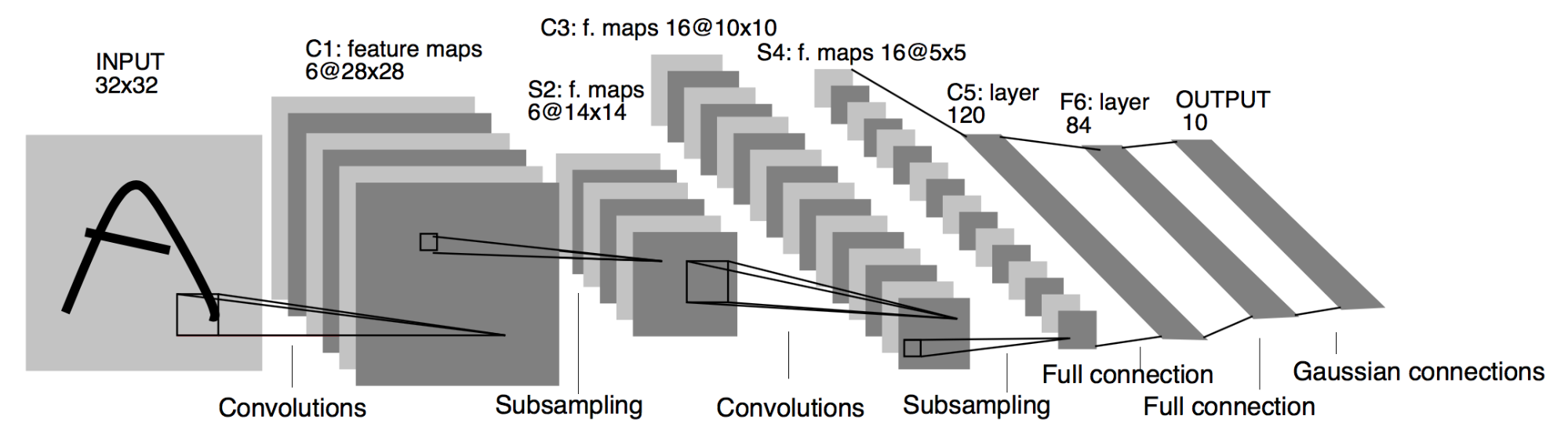
CNN

A convolutional neural network (CNN) consists of an output, input, and a variable number of hidden layers. The hidden layers of a CNN typically consist of convolutional layers, activation functions, pooling layers, fully connected layers and/or normalization layers. CNN have found great success in vision and sound applications.

Training a CNN on data from Cough Collection 1

Procedure

The cough dataset was loaded into memory and padded to make data the same size. Padding is required to match the cough size to the input size of the CNN. The data set was then split into training and test sets. Data augmentation was then applied only to the training set. The FFT magnitude(FFT squared feature) was extracted from both training and test sets. The training and test sets were then normalized independently. The training data was used to train the CNN while the test data was used to validate that the model can correctly classify samples it has not been trained on.

The CNN model used performs well on similar classification tasks. The Cough Collection 1 dataset was split randomly into training and validation sets 5 times to create 5 training and validation data sets. The CNN was trained and validated independently on each of the 5 training and validation sets

Results

• Average prediction accuracy is 56.66 % when evaluated against the test set
• Prediction accuracy (56.66%) is not much better than a random guess (50%)

Conclusions

• Not enough samples for the model to differentiate between Wet and Dry coughs.
• Similar applications use 100’s to 1000’s of samples.
• More samples are needed to properly evaluate the performance of the CNN

Examining one CNN training run on Cough Collection 1

To gain some insight into why the CNN had failed to label coughs correctly over five experiments, the details of one experiment were examined. The graph below is a comparison of the CNN prediction accuracy between the training data and the test data. The CNN shows improvement in prediction accuracy on the training set as the number of training runs(epochs) increases. This implies the CNN can correctly recognize coughs it has previously seen. Conversely, the CNN does not show any notable improvement on the testing data with increasing training runs. The CNN can not correctly label coughs it has never seen before. A high prediction accuracy on the training set with a low prediction accuracy on the testing set is a consequence of overfitting the training set.

Training on cough collection 1 plus 7 more samples from cough collection 2

Once data from Cough Collection 2 began to come in, the experiment was rerun with all the coughs from Cough Collection 1 and 7 Cough samples from Cough Collection 2. As more training data is provided to the CNN, it is expected that the prediction accuracy on the testing data set will begin to improve with increasing training runs (epochs).

Results

As samples are added the prediction accuracy of the CNN on the testing data is increasing with increasing training runs. This implies that the CNN is starting to learn more generalized features as more cough samples are provided. The accuracy is still very low but, the total number of training samples is very low as compared to similar applications.

Hyper Parameter tuning

Hyper parameters are variables that are not learned during training but can have a large effect upon performance. Hyper parameter tuning is performed by training the CNN with various parameter value combinations and comparing the results between runs. Even with a small number of hyperparameters, the number of possible combinations can become quite large. This precludes manual hyper parameter tuning as a realistic option. Automatic tuning can be done with a framework such as Talos. The CNN was trained on all available samples from Cough Collection 1 & 2. Heavy data augmentation was used to increase the training set size to the same level as used in comparable applications. The augmented data formed about 84% of the training data. Using Talos, 400 CNNs were trained with various hyper parameter combinations. The best performing network parameters were selected from the table generated by Talos. A subset of the hyper parameter table is shown below.

Subset of the hyper parameter search table

Conclusions

• It is possible to separate wet and dry coughs into two distinct sets with software
• There are frequency differences between wet and dry coughs.
• Algorithms appear to be improving with the addition of more samples

References

[1] Korpáš, J., Sadloňová, J., & Vrabec, M. (1996). Analysis of the Cough Sound: an Overview. Pulmonary Pharmacology, 9(5-6), 261–268. doi:10.1006/pulp.1996.0034

[2] Rizal, A., Hidayat, R., & Nugroho, H. A. (2015). Signal Domain in Respiratory Sound Analysis: Methods, Application and Future Development. Journal of Computer Science, 11(10), 1005–1016. doi:10.3844/jcssp.2015.1005.1016

[3] Chatrzarrin, H., Arcelus, A., Goubran, R., & Knoefel, F. (2011). Feature extraction for the differentiation of dry and wet cough sounds. 2011 IEEE International Symposium on Medical Measurements and Applications. doi:10.1109/memea.2011.5966670

[4] Ahmad, J., Muhammad, K., & Baik, S. W. (2017). Data augmentation-assisted deep learning of hand-drawn partially colored sketches for visual search. PLOS ONE, 12(8), e0183838. doi:10.1371/journal.pone.0183838

[5] 857389211010878. “KNN (K-Nearest Neighbors) #1.” Towards Data Science, Towards Data Science, 8 Nov. 2018, towardsdatascience.com/knn-k-nearest-neighbors-1-a4707b24bd1d.

[6] Weng, Sheng, and Sheng Weng. “Automating Breast Cancer Detection with Deep Learning.” Insight Data, Insight Data, 13 June 2017, blog.insightdatascience.com/automating-breast-cancer-detection-with-deep-learning-d8b49da17950.

John W Grun

Abstract

In this paper, a manually implemented LeNet-5 convolutional NN with an Adam optimizer written in Numpy will be presented. This paper will also cover a description of the data used to train and test the network,technical details of the implementation, the methodology of training the network and determining hyper parameters, and present the results of the effort.

Introduction

LeNet-5 was created by Yuan Lecun and described in the paper “Gradient-Based Learning Applied To Document Recognition” . LeNet-5 was one of the first convolutional neural networks used on a large scale to automatically classify hand-written digits on bank checks in the United States. Prior to LeNet, most character recognition was done by using feature engineering by hand, followed by a simple machine learning model like K nearest neighbors (KNN) or Support Vector Machines (SVM). LeNet made hand engineering features redundant, because the network learns the best internal representation from training images automatically.

This paper will cover some of the technical details of a manual Numpy implementation of LeNet-5 convolutional Neural Network including the details about the training set, structure of the lenet-5 CNN, weights and biases initialization, optimizer, gradient descent, the loss function, and speed enhancements. The paper will also cover the methodology used during training and selecting hyperparameters as well as the performance on the test dataset.

Related work

There are numerous examples of numpy implementations of LeNet 5 found across the internet but, none with more significance than any other. Lenet-5 is now a common architecture used to teach new students fundamental concepts of convolutional neural network

Data Description

The MNIST database of handwritten digits, contains a training set of 60,000 examples, and a test set of 10,000 examples. Each example is a 28 x 28 pixel grayscale image.
All training and test examples of the MNIST were converted from gray scale images to bilevel representation to simplify the function the CNN needed to learn. Only pixel positional information is required to correctly classify digits, while grayscale offers no useful additional information and only aids in increasing complexity. The labels of both the test and training examples were converted to one hot vectors to make them compatible with the softmax output and cross entropy loss function. Both indexes of the training and test sets were further randomized to ensure each batch was a random distribution of all 10 classes.

Model Description

Structure

The model is a implementation of LeNet 5 with the following structure:

• Input 28 x 28
• Convolutional layer (Pad = 2 , Stride = 1, Activation = ReLu, Filters = 6, Size = 5)
• Max Pool (Filter = 2, Stride = 2)
• Convolutional layer (Pad = 0 , Stride = 1, Activation = ReLu, Filters = 16 )
• Max Pool (Filter = 2, Stride = 2)
• Convolutional layer (Pad = 0 , Stride = 1, Activation = ReLu, Filters = 120)
• Fully Connected ( Size = 120, Activation = ReLu)
• Fully Connected (Size = 84, Activation = ReLu)
• Soft Max ( 10 Classes )

Weight and bias initialization

Since the original lenet-5 predates many of the more optimal weight initialization schemes such as Xavier or HE initialization, the weights were initialized with numpy random.randn while biases were zero filled with numpy zeros.

Optimizer

At first a constant learning rate optimizer was used for this network but, stable convergence required a very small learning rate. This small learning rate required a very long training time to achieve a reasonable accuracy on the test set. The constant learning rate optimizer was replaced with a numpy implementation of the ADAM optimizer. ADAM allowed for the use of higher learning rate that resulted in quicker and smoother convergence. The formulas that describe ADAM are shown below:

Gradient Descent

This implementation of LeNet-5 uses Mini-batch gradient descent. Mini-batch gradient descent is a trade-off between stochastic gradient descent (training on 1 sample at a time) and gradient descent (training on the entire training set). In mini-batch gradient descent, the cost function (and therefore gradient) is averaged over a small number of samples. Mini batch gradient descent was selected due to its increased convergence rate and the ability to escape local minimum.

Loss function

LeNet 5 produces a 10 class categorical output representing the numbers 0 to 9. The original LeNEt-5 used Maximum a posteriori (MAP) as the loss loss function. Cross-entropy was chosen as the loss function in this implementation instead of MAP since cross entropy appears to be the dominant loss function for similar classification problems and source code was available to check against. The formula for cross entropy loss is given below:

Speed Enhancements

To train the CNN in a reasonable amount of time several performance enhancements had to be made.

The python profiler was used to identify locations in the code that would have the largest effect on performance. The convolutional and max pooling layers consumed the majority of the running time. The running time of the convolutional and max pool layers was decreased by first converting the single threaded functions into multithreaded functions. Processing was divided up equally across the number of threads. Once threading was confirmed to be working properly, the Numba Just in Time compiler (JIT) was employed to convert python functions into native code. Numba JIT was then liberally applied throughout the code. These enhancements reduced the training time from over 1 day to a few hours, constituting a 6-8x speed up on average.

Method Description And Experimental Procedure

The LeNet 5 model implementation was trained on the MNIST dataset. After each training, the training loss versus epoch was plotted. The learning rate was decreased until the training loss vs epochs was a monotonically decreasing function. The number of epochs was selected to minimize the training loss while the training loss continued to decrease with every training epoch. Adjustments to the epochs sometimes also required adjustments to the learning rate to keep the training loss vs epoch a monotonically decreasing function.
In addition to the training loss, the prediction accuracy was computed. The accuracy was computed by the following method:
The input images were forward propagated through the network with the weights and biases learned during training. The class with the largest magnitude was selected as the prediction. The predicted class was compared to the label for a given input image. The percentage of correct predictions was computed across all input images forward propagated through the network.
The prediction accuracy was computed for both the training and testing sets . In a well trained network (one not underfitting or overfitting ) the test prediction accuracy should be close to the training prediction accuracy. If the training prediction accuracy is far greater than the test prediction accuracy it is a sign the network is overfitting on the training data and failing to generalize well.
The batch size was selected primary upon the cache limitations of the processor. A batch size of around 32 was determined to be small enough to fit in cache while also large enough to reduce overhead from thread context switching.

Results

Hyper parameters

The hyper parameters for this numpy implementation of LeNet 5 are as follows:

• Epochs = 20
• Learning rate = 0.0002
• Batch = 32

Training time

The total training time was brought down from 26 hours to train on the entire training set of 60000 examples to only 2.75 hours after applying speed enhancements.

Training loss

The training loss of LeNet-5 as plotted over 20 epochs. The training loss is monotonically decreasing indicating the network is effectively learning to differentiate between the ten classes in the MNIST dataset.

Accuracy

Accuracy on test set = 95.07%
Accuracy on Train set = 94.90%
The Lenet-5 implementation achieved a high accuracy on the test and train sets without a significant difference in prediction accuracy between the train and test sets which would be an indication of overfitting.

Conclusion

A Lenet 5 Convolutional Neural Network has been implemented only using Numpy that yields prediction accuracies over 95% on the test set. The network was trained on all 60000 examples found in the MNIST dataset and tested against the 10000 examples in the MNIST test set. The network used the standard LeNet Architecture with modifications where required. To decrease convergence time, a numpy ADAM optimizer was written. Several speed enhancements such as multi threading and just in time compilation were employed to decrease training time to a reasonable period.

References

[1] Lavorini, Vincenzo. “Speeding up Your Code (4): in-Time Compilation with Numba.” Medium, Medium, 6 Mar. 2018, medium.com/@vincenzo.lavorini/speeding-up-your-code-4-in-time-compilation-with-numba-177d6849820e.
[2] “Convolutional Neural Networks.” Coursera, www.coursera.org/learn/convolutional-neural-networks.
[3] LeCun, Yann. MNIST Demos on Yann LeCun’s Website, yann.lecun.com/exdb/lenet/.
[4] Lecun, Y., Bottou, L., Bengio, Y., & Haffner, P. (1998). Gradient-based learning applied to document recognition. Proceedings of the IEEE, 86(11), 2278–2324. doi:10.1109/5.726791
[5] “MNIST Database.” Wikipedia, Wikimedia Foundation, 11 Apr. 2019, en.wikipedia.org/wiki/MNIST_database.
[6] “Cross Entropy.” Wikipedia, Wikimedia Foundation, 8 May 2019, en.wikipedia.org/wiki/Cross_entropy.
[7] “Stochastic Gradient Descent.” Wikipedia, Wikimedia Foundation, 29 Mar. 2019, en.wikipedia.org/wiki/Stochastic_gradient_descent.

Materials

The entire frame is build from 1in x 1in x 24in 80/20 T slot. These can be obtained from https://www.mcmaster.com/

The rails are joined with a combination of “Flanged Button Head Screws”, T slot nuts, and tapped ends. Any Tslot end that had to connect to another Tslot at a 90 degree angle had it’s end tapped with a 1/4-20 tap. The cooresponding Tslot to be joined had an access hole drilled 1/2 in from the end. This access hole allows me to tighten “Flanged Button Head Screws” with a hex wrench.

Filename: 20180621_192035.png
Description: A collection of cut aluminum extrusions laid out on the floor, the materials being prepared for the frame of the CNC machine.

Picture of the drill holes on the bottom front of the frame.

Base

The types of Tslot used to build the frame. 1in x 1inx 24in and 1in x 2in x 24in. The frame X and Y dimensions are 24in x 26in. This dimesion was choosen to encompass the entire CNC while also requiring minimal cuts.

The CNC was bolted directly to the 1in x 2in x 24 rails. The 2in dimesion is vertical as to resist bending due to the weight of the CNC ~120lbs.

Top Enclosure Frame

The top of the enclosure frame will slide with the X axis back and forth. This allows me to compress the size of the overall frame without losing the protection of a fully enclosed machine. This is a 3d printed 80/20 linear bearing. I printed this in PLA. With the addition of some greese it slides very easily even under load.

3D Printed 80-20 bearing.

Profile shot of the 80-20 bearing

3d printed 80-20 bearing with a screw and tslot nut.

3d printed 80-20 bearing mounted on the base.

The bottom rail of the top enclosure will slide on these 80-20 bearings. The X/Y table of the CNC will be connected to the Top enclosure. This will shift the frame along with the Y axis. The axis of the CNC table will move inside the top enclosure.

View of the top frame before connecting the X axis to the enclosure

Shifting the top enclosure to on side.

X/Y Table to Top Enclosure connection

3D Printed connections and spacers.

Tslot and Tslot brackets that will connect the X/Y table to the Top Enclosure Frame.

Motor side

Top view of the X/Y table to Top Enclosure connection.

A close-up shot of an aluminum profile with a sliding component. It seems to show the assembly of one of the axes, using standard T-slot extrusion for mounting and moving components.

Side view of the X/Y table to Top Enclosure slide connection.

End view of the X/Y table to Top Enclosure slide connection. The 80-20 bearing is clearly seen in the Tslot. The Tslot rail is part of the Top Enclosure.

Connecting the motor side of the x/Y table to the Top Enclosure. The white 3d Printed spacer is required to make everything fit correctly.

Another angle. Dry fitting before we physically connect the slide to the X/Y table.

The AL block is the end of the X/Y table. The large hole is where the motor for the y axis passes. The motor mounts to the other side. The bracket faces the inside towards the CNC machine when mounted.

We are aligning the slide connection to the AL motor block and marking the bolt positions with a punch.

I used a center drill to start the mounting holes.

Picture to show alignment of the holes to the connection bracket.

Drilled out the mounting holes with a #7 drill bit. We will be tapping these with a 1/4-20 tap.

The block is joined to the frame with a 80-20 linear bearing(white) this allows the component to move along the rail in the direction of y axis movement. The AL bracket is obsured by the AL motor mount block.

Linear bearing shown in rail that forms the bottom of the top enclosure.

Rail mounted in enclosure and the AL mounter mount block reattached to the CNC X/Y table.

Non motor side

I tapped 2 holes into the non motor side end of the X/Y table. This will allow us to attach a tslot section. Each hole is 1/2 in from the edge in both X and Y.

AL bracket with Tslot nuts. Side view

AL bracket with Tslot nuts. Bottom view.

Marking access hole. 1/2 in from the end. This will allow us to tighten the screws above.

1/4 in access hole drilled.

Attaching the spacers to the X/Y non motor end.

Both sides mounted.

Reattaching the X/Y non motor end to the X/Y table.

A side view of a linear guide and spacer assembly.

Linear 80-20 slide in frame.

Connecting the X/Y table non motor side to the bottom of the Top Enclosure Frame.

View of linear bearing on the non motor side. The linear bearing slides inside the rail.

Both Sides of the X/Y table attached to the frame. The Y axis moves front to back within the frame while the x axis moves the top frame left to right.

CNC moving.

Wiring

Spindle Control

Rerunning the spindle control wiring

Wiring junction for the X/Y table endstops

End stop wiring and stepper motor signals. All twisted pairs to reduce noise.

Testing with Linuxcnc.

Inside power switch and Estop enclosure.

Inside power switch and Estop enclosure.

Power switch and E-Stop wiring in box.

The control electronics, end switches, and power supplies will be covered in other posts.

Ubuntu Watch filesystem limit Work Around

In the terminal run

sudo gedit /etc/sysctl.conf

fs.inotify.max_user_instances=524288
fs.inotify.max_user_watches=524288
fs.inotify.max_queued_events=524288

Reboot for changes to take effect.

John Grun

Abstract

In this paper, we introduce the Peer to Peer Network Domain Name System (P2PN-DNS) a distributed implementation of the
Domain Name System (DNS) that hopes to offer solutions to shortcomings of the current DNS such as susceptibility to outages while mitigating attempts of domain name censorship, and provide a fault tolerant name lookup service for software containers that is independent of upstream servers. Performance metrics including the time to reach consistency between nodes, service availability in lieu of loss of nodes, and average response time to DNS queries will be examined.

I. Introduction

The Domain Name System (DNS) is a critical element of internet infrastructure that associates IP addresses to human readable domain names. E.g Google.com is located a IP:172.217.6.238. When DNS was introduced in 1987 with the RFC 1034 /RFC 1035 17/18 standards, the internet consisted of relatively few computers where a simple hierarchical tree model functioned well.
As the internet scaled, DNS was expanded to accommodate the exponential growth in computers. In this regard, DNS has been a tremendous success but, it is not without serious flaws, most notably respectability to attacks on or failures of the Root DNS servers. A Root DNS Server acts as the authoritative source for the entire network.

Figure 1: DNS tree structure ²⁴

In part due to the tree structure of DNS, there are only thirteen DNS Root Servers in the world. An attacker only needs to target a few DNS root servers to cripple IP address to domain name translation in an entire region effectively blocking internet access for most users. Attacks against DNS Root Servers have occurred and appear to be becoming more frequent from various entities, such as hackers, or state actors. It is also quite conceivable that DNS would be a target in wartime. Additionally, centrally located servers are vulnerable to regional events such as power outages or natural disasters.

Another issue that has been seen in the wild is the censorship of websites by state, corporate, or other actors via DNS poisoning. DNS poisoning blocks access to websites by disrupting the domain name lookup between a DNS resolver and the regional DNS server. E.g Google.com is located at IP:172.217.6.238. China ²⁶ and Iran ²⁵ have both used DNS poisoning to block access to internet domains. Corporations such as Charter, Comcast, and Optonline ³ have used DNS poisoning to reroute search results away from competitor websites or to collect advertising profits.

An additional limitation of the existing DNS system is a lack of software container support.
Existing DNS solutions for software containers either rely upon a DNS repeater or upon a standard DNS server. These methods simply extend the existing DNS system. If the upstream DNS is made inoperable or poisoned, the containers will be affected as well. This dependency upon existing DNS introduces a single point of failure into what would otherwise be fault tolerant architecture.

The aforementioned problems encountered are a consequence of the centralized hierarchical architecture of DNS. A different architecture can be defined to address these problems while providing the same functionality. We propose to build a decentralized Peer to Peer Network DNS (P2PN-DNS) that will not rely on central servers. We intended to take the best practices from existing distributed robust protocols such as bitTorrent and bitcoin to accomplish our goal. Also, each P2PN-DNS node should be able to contain an internal store of the domain name IP address relations without relying on additional software or servers.

II. Related and Previous Work

There have been several different methods over the years to address some or all of the aforementioned problems with DNS.

Amazon Web Services (AWS) offers a implementation of DNS known as Amazon Route 53. Route 53 is believed to be a distributed DNS system but, architectural details have not been forthcoming from Amazon.²⁷

Another project DC/OS, (the Distributed Cloud Operating System) contains an internal DNS repeater. While the DC/OS DNS repeater is distributed on the internal network and consists of multiple nodes, it is not a true distributed peer to peer DNS. The DC/OS DNS is a redundant DNS system that acts as a DNS forwarder from a DNS server further up the DNS tree making it vulnerable to the same issues as DNS.28 See https://dcos.io/

A third related work, Kad Node claims to be a small peer to peer DNS resolver or to act as a DNS proxy. Kad node stores DNS records in a distributed hash table, similar to our proposal but, it differs in that it does not appear to utilize a hash based DNS update ordering scheme. At the writing of this paper Kad Node appears to be inactive. ²⁹ See Kad Node at https://github.com/kadtools/kad

III. Contribution

Technical Problems

The main technical concerns affecting a distributed DNS are the same as those encountered in any system where information is distributed between disparate nodes, namely data consistency, availability, and network partition tolerance. As stated by the CAP (Consistency, Availability, and Partition Tolerance) theorem, it is impossible for a distributed data store to simultaneously provide all three of the guarantees of consistency, availability, and partition tolerance at any given time. This implies compromises must be made between the three. In the case of a distributed DNS the decision as to which guarantees to support and which to neglect is relatively straight forward. In a real world environment, computers crash, network connections fail, and infrastructure can be disabled, thus network partition tolerance is a requirement of any realistic distributed DNS. As a critical service of internet infrastructure, DNS must be always available for the internet to operate properly. Thus availability is a required guarantee as well.

With partition tolerance and availability as required guarantees, continuous consistency becomes impossible to guarantee according to the CAP theorem. In the case of DNS, continuous consistency is not a requirement and eventual consistency is more than sufficient. In fact, currently a DNS record updates are eventually consistent and can take up to 24 hours to complete.

Partition tolerance and availability can both be addressed by designing each node to operate independently of all the others on the network. The independent nodes need only exchange update information to ensure eventual consistency of the DNS records. In this architecture, the more nodes added to a network, the more reliable the system will become.

In a distributed system relying upon eventual consistency to make data agree across nodes, the issue of order of updates arises, since there is the possibility of updates arriving at other nodes in a different order than they must be applied to ensure agreement between nodes.
This can be addressed by writing updates to a commit log prior to writing the DNS update. A commit log is a data structure that keeps track of the operations to be performed in first in first out (FIFO) order. When a new DNS record update is received by a node, the update is first written to the commit log. While changes are in the commit log, actions can be taken to ensure the correct ordering of the updates. The ordering of the commits can be verified and corrected by comparing timestamps or by using a hashing based scheme. An update will only be removed from the commit log once the node has finished updating the DNS record.

Figure 2: Commit Log Functionality ¹⁶

There are some properties of DNS record updates that allow for some simplifications.
Since the update history of each domain name in DNS is independent of all other domain names, we do not need to ensure ordering between different domain names. This property can be utilized to simplify the consistency requirement since it greatly limits the amount of possible combinations in ordering. We need only establish an update chain on a per domain name basis.
The update history can be established with timestamping. Each update is time stamped, and if every node is synced to the same clock the order of updates can be ordered correctly. If the nodes do not have a common clock source this method fails to guarantee the correct update ordering. This ordering problem is what data structures and algorithms such as Merkle trees and blockchains were developed to solve. A Blockchain or Merkle tree takes a hash of a data record, then the next data update in line is a hash of the new update combined with the previous hash. The update received by a node can be confirmed ordered correctly by hashing the previous hash with the current update and comparing the result. If the hash is the same, the DNS record can be updated. If the hash is incorrect a Quorum can be called to reach a consensus between nodes. Since a record update is only concerned about the most recent update and is not dependent upon the entire history of the update chain the ordering requirement can be relaxed to only include the last few updates. In this case, a Quorum can serve the purpose of correcting out of order entries. This situation may arise if some nodes do not receive a DNS update or network issues cause updates to arrive in the wrong order.

The next technical challenge is how to store the DNS records. Since DNS are retrieved based upon the domain name, the most logical method is a simple key value store, where the domain name is used as the key and the corresponding ip address is the value.

Another issue that arises in the real world is the need to automatically find peers. In a small scale system, manually assigning peer address is possible but, as the system scales this method quickly becomes untenable. Nodes must employ a method to locate each other without the intervention of humans. One such method that has proven to be quite effective in other distributed applications is the distributed hash table (DHT). A distributed hash table (DHT) provides a lookup service similar to a hash table: (key, value) pairs are stored in a DHT, and any participating node can efficiently retrieve the value associated with a given key. Responsibility for maintaining the mapping from keys to values is distributed among the nodes, in such a way that a change in the set of participants causes a minimal amount of disruption. This allows a DHT to scale to an extremely large numbers of nodes while handling continual node arrivals, and departures.

Figure 3: Distributed Hash Table Functionality ¹⁵

Possibly the hardest technical problem to address in a distributed system is known as the “Trust Problem.” The trust problem brings forth the question of which node is friendly, and which is malicious. If this implementation was utilized on the open web, the trust problem can be addressed with strategies such as proof of work as employed by technologies such as Blockchain. Nevertheless, if only running on a isolated network, methods such as trusted tokens would are viable. This problem is beyond the scope of this paper but, the authors felt it was important enough to mention and it will have to be addressed in future releases.

IV. Algorithm and Implementation

The implementation of P2PN-DNS involved the union of several aforementioned key concepts in distributed computing, the key-value store, distributed hash table, and the commit log.

Figure 4: Implementation Block Diagram

At the most basic level DNS can be viewed as a key value store where the domain name serves as the key and the IP address serves as the value. In practice, the DNS domain name to ip address relation is called a resource record and may contain a plethora of data including IP address, CNAME, TXT, etc. For our demonstration only a simple domain name to ip address was implemented.

The main data structure enabling P2PN-DNS is the distributed hash table. In theory a distributed hash table appears simple but, in practice the implementation of the data structure and overlay network can be very labor and time intensive. There was no reason to reinvent the wheel for P2PN-DNS so, OpenDHT was used for the DHT. OpenDHT aligns well with the scope and goals of P2PN-DNS while bundling in support for other desirable features such as IPv4 and IPv6, public key cryptography, distributed shared keys, and an overall concise, and clear approach. OpenDHT can be found at https://github.com/savoirfairelinux/opendht

Since OpenDHT was originally targeted similar distributed applications, the key-value store and commit log functionality were already present and did not have to be implemented independently.

The other major facet of P2PN-DNS was the implementation of the DNS protocol. DNS protocol support was based upon a bare bones implementation of DNS called SimpleDNS. The C source code had to be heavily modified to make it compatible with the C++ elements of P2PN-DNS. Most eventenly the use of C++ 11 std::function as callbacks. Additionally, the DNS update (22) message had to be implemented. The DNS update (22) message did not become a public facing feature in the current DNS system and as such it is not included in most DNS resolvers. Systems that do implement a DNS update scheme are called Dynamic Dns or (DDNS) and have accompanying attenication to update a DNS record. (DDNS) is not directly compatible with standard DNS and relies upon an authoritative entity to make the DNS update to the rest of the Domain Name System. In the interests of time and simplicity, a minimal DNS update scheme was implemented. This shortcoming will be rectified in future releases. Please see for the original SimpleDNS source code at https://github.com/mwarning/SimpleDNS

The ordering of the updates is determined strictly based upon timestamp in this release. This timestamp method works as long as all the nodes are time synced. This is not a valid assumption in a real world environment as nodes may be operating on seperate networks with differing time sources. In future releases a hash bashed ordering scheme as mentioned in Section 3 will be investigated.

The source code for the P2PN-DNS and further documentation can be found at: https://github.com/P2PN-DNS/P2PN-DNS

V. Results and Analysis

Experiment and Evaluation

There are a few metrics that matter in a real world application such as the response time to DNS queries, service availability in lieu of loss of nodes, and the average time required to sync records across nodes. For our experiments we propose to examine these metrics and compare, where applicable, to the current DNS system. Dnsmasq will serve as the comparison benchmark as it is a widely deployed DNS forwarder for DNS queries.

To measure the response time of the nodes to a DNS request, a DNS request was sent to a P2PN-DNS node via the dig utility, and the record response was recorded. The time taken from request to response was recorded by Wireshark. The same method was employed against DNS(dnsmasq). Five common domain names were chosen; google.com, Amazon.com, Nytimes.com, alibaba.com, and stackoverflow.com. Three samples were taken for each domain name on both P2PN-DNS and dnsmasq to establish a trend and to compensate for outliers. This resulted in 15 queries per dnsmasq and 15 queries for P2PN-DNS. Dnsmasq was running on same network as P2PN-DNS. P2PN-DNS records were added via the DNS update message prior to running the experiment.

Figure 5: Query Response Times of DNS versus P2PN-DNS

The first request for each domain name to Dnsmasq was of longer duration.This was due to Dnsmasq requesting current information from a higher tier DNS server( Google DNS 8.8.8.8). The second and third requests were served from the Dnsmasq local cache, hence the much shorter duration in response time. P2PN-DNS had slightly longer response time than the Dnsmasq cached response but, less than the first non cached result. This behavior was to be expected as P2PN-DNS has to search the DHT on every lookup and currently does not have local caching enabled. Response time of P2PN-DNS could be improved by enabling local caching in future releases.

To test to the availability of P2PN-DNS in lieu of loss of nodes, is to observe the behavior of the P2PN-DNS nodes when nodes disappear from the network. To conduct this experiment, five nodes were started. A DNS record update message was sent to one of the nodes. The nodes were allowed to reach a consistent state where all nodes are informed of the updated record as observed by querying each node for the updated record. One node was be taken offline at a time. Each time a node was removed, the DNS records were checked for consistency between the remaining nodes.

Figure 6: Progression of loss of nodes to test availability

The DNS record was returned correctly even after only one node of the original five remained. This shows that the P2PN-DNS can fulfill the availability and partition tolerance guarantees even as nodes are removed from the network.

To observe the amount of time required to sync records across nodes, the timestamp in the commit log was compared between two different nodes. The difference in the arrival timestamp between the two nodes is directly correlated to the time required to sync records. To ensure accurate timestamping, all nodes were tied to an common clock and synced with Network Time Protocol (NTP).

Figure 7: Syslog output from two nodes

In the figure above, the syslog output of two nodes can be observed. To produce these results, a DNS update packet was sent to one node. Syslog was monitored for logs containing information about the record update between the two nodes. The update to a record can be seen in one node and in less than one second later, the update is available on the other node. Network capabilities have an impact on the overall record sync time and can affect time jitter. The network variability(jitter) timing issue was avoided by running the nodes on the same network with a common NTP server.

VI. Conclusion

With our implementation of a distributed DNS we were able to find a workable tradeoff between consistency, availability, and partition tolerance. By conducting thorough experiments and analysis, we showed that P2PN-DNS can guarantee eventual consistency, high availability, and partition tolerance while also providing a comparable amount time required to process DNS queries as compared to existing DNS solutions such as DNSmasq. P2PN-DNS was shown to be available even as nodes were removed giving credence to the claim that P2PN-DNS would be less susceptible than current DNS to regional outages or purposeful attacks.
Additionally, the distributed nature of P2PN-DNS makes it applicable for software containers which would benefit from a fault tolerant solution such as P2PN-DNS.

VII. References

[1] “Domain Name System”. En.wikipedia.org. N.p., 2017. Web. 2 November 2017.https://en.wikipedia.org/wiki/Domain_Name_System
[2] “Distributed Denial of Service Attacks on Root Nameservers ”. En.wikipedia.org. N.p., 2017. Web. 2 November 2017. https://en.wikipedia.org/wiki/Distributed_denial-of-service_attacks_on_root_nameservers
[3] “I Fought My ISPS Bad Behavior and Won”. Eric Helgeson. Web. 2 November 2017. https://erichelgeson.github.io/blog/2013/12/31/i-fought-my-isps-bad-behavior-and-won/
[4] Eckersley, Technical Analysis by Peter. “Widespread Hijacking of Search Traffic in the United States.” Electronic Frontier Foundation, 14 Oct. 2011. Web. 2 November 2017. https://www.eff.org/deeplinks/2011/07/widespread-search-hijacking-in-the-us
[5] “Transaction Log”. En.wikipedia.org. N.p., 2017. Web. 2 November 2017. https://en.wikipedia.org/wiki/Transaction_log
[6] “Merkle Tree”. En.wikipedia.org. N.p., 2017. Web. 2 November 2017.
https://en.wikipedia.org/wiki/Merkle_tree
[7] Kangasharju, Jussi. Chapter 4: Distributed Systems: Replication and Consistency. N.p., 2017. Web. 7 November 2017. https://www.cs.helsinki.fi/webfm_send/1256
[8] “Blockchain”. En.wikipedia.org. N.p., 2017. Web. 7 November 2017. https://en.wikipedia.org/wiki/Blockchain
[9] Jacquin, Ludovic, et al. “The Trust Problem in Modern Network Infrastructures.” SpringerLink, Springer, Cham, 28 Apr. 2015. N.p., 2017. Web. 7 November 2017. https://link.springer.com/chapter/10.1007/978-3-319-25360-2_10
[10] “ACID”. En.wikipedia.org. N.p., 2017. Web. 8 November 2017. https://en.wikipedia.org/wiki/ACID
[11] DataStax Academy Follow. “A Deep Dive Into Understanding Apache Cassandra.”LinkedIn SlideShare, 25 Sept. 2013. N.p., 2017. Web. 2 December 2017. https://www.slideshare.net/planetcassandra/a-deep-dive-into-understanding-apache-cassandra
[12] “Peer-to-Peer (P2P) Systems.” SlidePlayer. N.p., 2017. Web. 2 December 2017 http://slideplayer.com/slide/4168557/
[13] “Non-Transitive Connectivity and DHTs “https://www.usenix.org/legacy/events/worlds05/tech/full_papers/freedman/freedman_html/index.html
[14] “Amazon Route 53”. En.wikipedia.org. N.p., 2017. Web. 6 December 2017.
https://en.wikipedia.org/wiki/Amazon_Route_53
[15] “Distributed hash table” .En.wikipedia.org. N.p., 2017. Web. 6 December 2017. https://en.wikipedia.org/wiki/Distributed_hash_table
[16] “FIFO (computing and electronics)” .En.wikipedia.org. N.p., 2017. Web. 6 December 2017. https://en.wikipedia.org/wiki/FIFO_(computing_and_electronics)
[17] “RFC 1034 DOMAIN NAMES - CONCEPTS AND FACILITIES”, N.p., 2017. Web. 2 November 2017. https://www.ietf.org/rfc/rfc1034.txt
[18] “RFC 1035 DOMAIN NAMES - IMPLEMENTATION AND SPECIFICATION” , N.p., 2017. Web. 2 November 2017. https://www.ietf.org/rfc/rfc1035.txt
[19] “Embedded DNS server in user-defined networks” N.p., 2017. Web. 2 November 2017. https://docs.docker.com/engine/userguide/networking/configure-dns/
[20] “OpenDHT” Web. 2 November 2017. https://github.com/savoirfairelinux/opendht
[21] “SimpleDNS: Web. 2 November 2017. https://github.com/mwarning/SimpleDNS
[22] “ Dynamic Updates in the Domain Name System (DNS UPDATE)” Web. 2 November 2017. https://tools.ietf.org/html/rfc2136
[23] “ You can’t Peer to Peer the DNS”
https://nohats.ca/wordpress/blog/2012/04/09/you-cant-p2p-the-dns-and-have-it-too/
[24] “DNS Server”
https://gitlearning.wordpress.com/2015/06/23/dns-server/
[25] “Internet censorship in Iran” https://en.wikipedia.org/wiki/Internet_censorship_in_Iran
[26] “Great Firewall”
https://en.wikipedia.org/wiki/Great_Firewall
[27] “ Amazon Route 53”
https://en.wikipedia.org/wiki/Amazon_Route_53
[28] “DC/OS” https://dcos.io/
[29] “Kad Node” https://github.com/kadtools/kad